Gerrymandering
James Kitchens
May 28, 2024
Python
D3
In 2022 during a late night (couldn’t sleep) coding exploration, I wrote a small maze generator script in R. I was interested in pathfinding algorithms and specifically whether certain nodes in a graph are more likely to be traversed through than others. It may not be obvious but a maze can be reinterpreted as a graph (or network). Say we have a graph where the nodes are laid out in a square grid and connected to their direct neighbors. We can think of removing an edge between two nodes as placing a wall down between those positions in our maze. In both the graph and maze, this action means the same thing - traveling directly between those two positions is prohibited. If we continue to remove edges in the graph, while being careful to ensure that all nodes can still be reached by any other node, we eventually work our way down to a so-called spanning tree. A spanning tree is a tree which connects every single node in the graph without forming any loops (when a node is connected in multiple ways). Simple mazes like this all have an associated spanning tree, which is what is passed into the pathfinding algorithms to solve them. But why am I talking about some throw away code from over a year ago…
I was reading Shape: The Hidden Geometry of Information, Biology, Strategy, Democracy, and Everything Else by Jordan Ellenberg and in one of the last chapters, Ellenberg talked about gerrymandering and specifically the ReCom algorithm developed by Deford, Duchin, and Solomon (2021) for dividing up a voting district. In essence, this algorithm uses graph theory to move through various districting configurations with the goal of finding a set which best fits desired criteria, such as population balance, contiguity, compactness, etc. The algorithm works on many of the same principles as my maze generator (which will become more obvious shortly) so I thought I would take a shot at expanding my script during a long weekend.
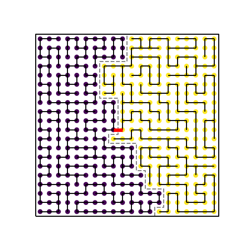
Cutting a spanning tree into districts. The spanning tree reaches every node within the square lattice graph. It is chopped at the central edge marked in red, resulting in the equally-sized purple and yellow districts. The grey line marks the boundary line between the districts.
The ReCom algorithm generates a spanning tree on a graph positioned within the bounds of the region that is to be divided. It then identifies the edge in the tree that when cut results in an equal number of nodes in the resulting two subtrees. Disappointingly, not all trees have an edge like this! I’m sure that there is some really interesting graph theory work on ways to identify when this is the case, though that extends beyond the scope of this exploration. In the case that there isn’t a central edge, the ReCom algorithm starts over from the beginning, generating a new spanning tree for the region, and tries again. In the event that there is a central edge, it chops that edge, resulting in two groups of connected nodes. These represent the two new districts.
gerrymandering.py
import networkx as nx
import matplotlib.pyplot as plt
from matplotlib import collections as mc
import random

def create_random_spanning_tree(g):
    tree = nx.create_empty_copy(g)
    num_nodes = g.number_of_nodes()
    visited = []
    node = list(g.nodes())[0]
    while len(visited) < num_nodes:
        if node not in visited:
            visited.append(node)
        neighbors = list(g.neighbors(node))
        possible_neighbors = [n for n in neighbors if n not in visited]
        if len(possible_neighbors) > 0:
            new_node = possible_neighbors[random.randint(0,len(possible_neighbors)-1)]
            tree.add_edge(node, new_node)
            node = new_node
        else:
            node = neighbors[random.randint(0,len(neighbors)-1)]
    return tree

def divide_into_two_districts(g):
    found = False
    while not found:
        tree = create_random_spanning_tree(graph)
        betweenness = nx.betweenness_centrality(tree)
        for k, v in sorted(betweenness.items(), key=lambda item: item[1], reverse=True)[:3]:
            if not found:
                for neighbor in tree.neighbors(k):
                    test = tree.copy()
                    chopped_edge = (k, neighbor)
                    test.remove_edge(k, neighbor)
                    groups = list(nx.connected_components(test))
                    if len(groups[0]) == len(groups[1]):
                        found = True
                        break
    districts = {}
    for i,group in enumerate(groups):
        for node in group:
            districts[node] = i
    return districts, tree, chopped_edge


dim = 20
graph = nx.grid_2d_graph(dim, dim)
districts, tree, chopped_edge = divide_into_two_districts(graph)
Though my original maze generator was written in R, I’ve been working with Python’s networkx library a lot recently and knew that it would have some helpful functions for this project, so I converted everything over to Python. I started by generating a square lattice graph using networkx.grid_2d_graph(). To identify a spanning tree, I initially used networkx.random_spanning_tree() but found it to be quite slow on large grids. My maze generator script was much faster (maybe because it doesn’t evenly sample spanning trees, I don’t know?), so I used that instead. Now armed with the spanning tree, I identify the central edge in the tree by filtering edges based on their betweenness and checking the most likely candidates. Similar to the ReCom algorithm, if this central edge does not exist, I generate a new spanning tree and try again.
gerrymandering.py
def determine_boundary(groups,dim):
    starts = []
    ends = []
    s = None
    for x in range(dim):
        for y in range(dim):
            if x != dim-1 and groups[(x,y)] != groups[(x+1,y)]:
                starts.append((x+0.5,y-0.5))
                ends.append((x+0.5,y+0.5))
                if y == 0:
                    s = (x+0.5,y-0.5)
                elif y == dim-1:
                    s = (x+0.5,y+0.5)
            if y != dim-1 and groups[(x,y)] != groups[(x,y+1)]:
                starts.append((x-0.5,y+0.5))
                ends.append((x+0.5,y+0.5))
                if x == 0:
                    s = (x-0.5,y+0.5)
                elif x == dim-1:
                    s = (x+0.5,y+0.5)
    if s == None:
        s = starts[0]
    boundary_line = [s]
    while len(boundary_line) <= len(starts):
        possible_new_s = []
        if s in starts:
            indices = [i for i,n in enumerate(starts) if n == s]
            possible_new_s.extend([ends[i] for i in indices])
        if s in ends:
            indices = [i for i,n in enumerate(ends) if n == s]
            possible_new_s.extend([starts[i] for i in indices])
        new_s = [ns for ns in possible_new_s if ns not in boundary_line]
        if len(new_s) > 0:
            boundary_line.append(new_s[0])
            s = new_s[0]
        elif (len(boundary_line) == len(starts)) and (boundary_line[0] in possible_new_s):
            boundary_line.append(boundary_line[0])
        else:
            print("FAIL")
            break
    return boundary_line


boundary = determine_boundary(districts, dim)
Since all of the nodes have a geographic position, it’s straightforward to then plot the districts and the boundary between them. To identify this boundary, I looped through every node and checked whether its neighbor was in the same district. If not, then I added a wall between the nodes. I then linked all of these walls together to get the continuous boundary line by following some assumptions that wouldn’t necessarily hold up in more complex cases, but luckily, we don’t need to worry about those here in this simple two district case.
gerrymandering.py
fig,ax = plt.subplots(figsize=(5,5))
boundary_line = mc.LineCollection([boundary], color="black")
ax.add_collection(boundary_line)
rim_line = mc.LineCollection([[(-0.5,-0.5),(dim-0.5,-0.5),(dim-0.5,dim-0.5),(-0.5,dim-0.5),(-0.5,-0.5)]], color="black")
ax.add_collection(rim_line)
plt.xlim(-1, 20)
plt.ylim(-1, 20)
ax.set_axis_off()
plt.savefig("districts.svg")
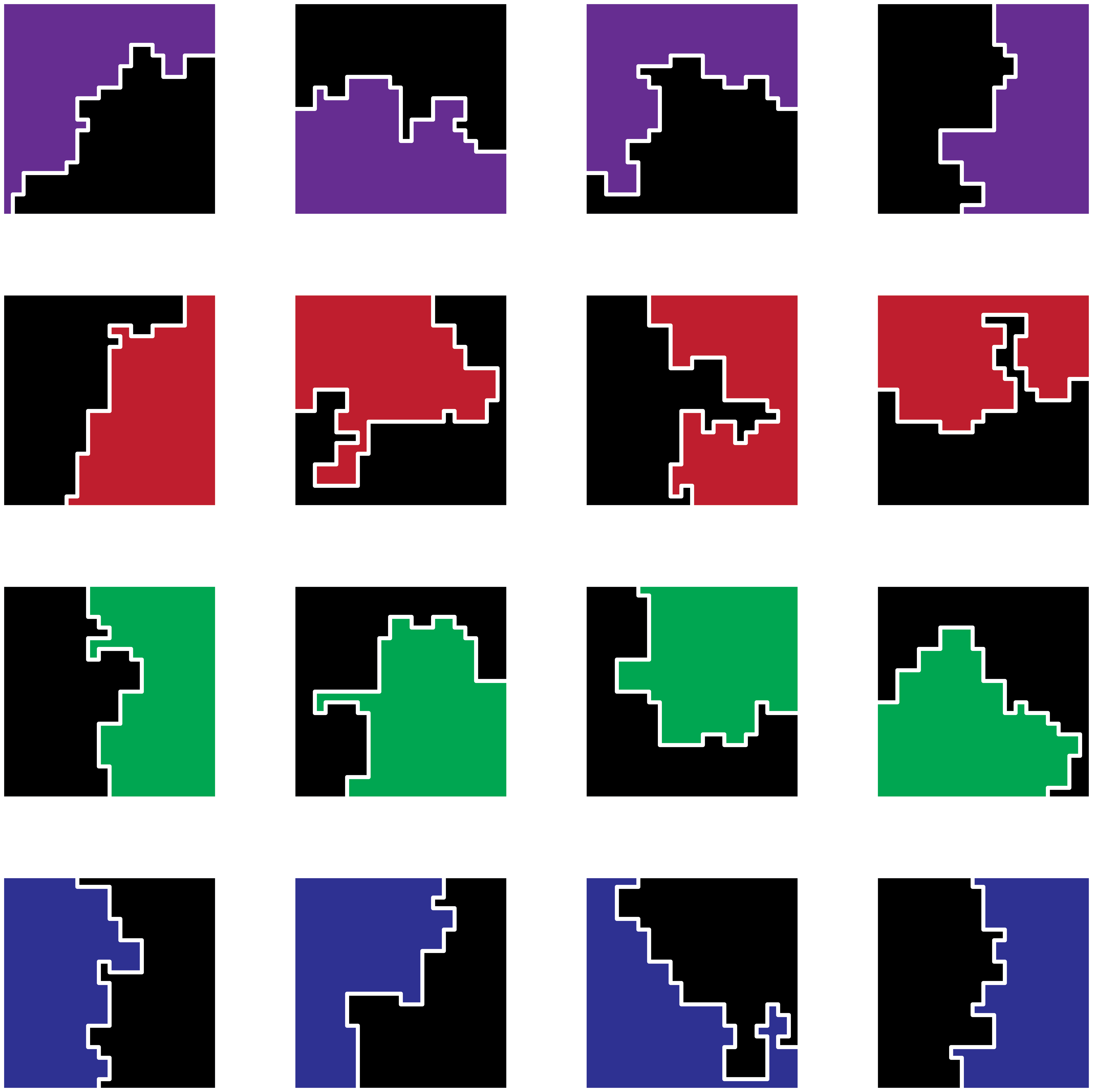
Collage of random districting results. Each subfigure is a separate run of the code. Colors are added only for styling.
I find it pretty interesting to just rotate through all of the ways that you can split up the region, with some cuts being quite straight and others being a bit more “organic”. The algorithm ensures that districts are contiguous shapes and under very unlikely circumstances it is possible that one district completely envelops the other (I’ve only seen this occur when I use a custom built spanning tree). My version of this algorithm only ensures that there is an equal number of nodes in each district, but you can see how you could add many more rules to ensure that the districts are balanced for other characteristics. At the top of this blog post, I’ve animated various districting cuts by exporting the SVGs of different runs and providing those paths to D3.js.
gerrymandering.html
<!DOCTYPE html>
<html lang="en">

<header>
    <meta charset="UTF-8">
    <title>Gerrymandering</title>
    <meta name="viewport" content="width=device-width,initial-scale=1">
    <script src='https://d3js.org/d3.v7.min.js'></script>
</header>

<body>
    <div class="images" style="max-width: 600px; margin: auto; padding: 25px;">
        <div id="districts"></div>
    </div>

    <script>
        //Adapted from https://observablehq.com/@onoratod/animate-a-path-in-d3
        // Create the SVG
        const svg = d3.select("#districts").append("svg")
            .attr("viewBox", "0 0 267.21 265.5");

        var outline = svg.append("path")
            .attr("d", "M51.6,313.8h265.7v-264H51.6V313.8")
            .attr("fill", "white")
            .attr("stroke-width", 2)
            .attr("stroke", "black")
            .attr("transform", "translate(-50.89 -49.05)");

        // Add the line
        var path = svg.append("path")
            .attr("fill", "none")
            .attr("stroke-width", 2)
            .attr("stroke", "black")
            .attr("transform", "translate(-50.89 -49.05)");

        const district_boundaries = [
            "M197.8,313.8v-13.2v-13.2h13.3v-13.2V261v-13.2v-13.2v-13.2v-13.2h13.3V195v-13.2v-13.2v-13.2h13.3v-13.2h13.3V129h-13.3h-13.3v13.2h-13.3v13.2h-13.3h-13.3v-13.2h-13.3h-13.3V129v-13.2h-13.3h-13.3h-13.3v-13.2h-13.3V89.4V76.2h13.3V63h13.3V49.8",
            "M250.93,49.8V63H277.5V76.2h13.29v39.6H211.07V89.4H171.21V76.2H131.36V89.4h13.28v26.4h13.29V129h13.28V115.8h26.58V129h13.28v13.2h13.29v26.4h39.85V155.4H277.5V142.2h13.29V195h13.28v13.2H277.5v13.2H264.21v13.2H237.64V221.4h13.29V195H237.64v13.2H211.07v39.6H184.5V234.6H171.21V221.4H157.93V195H118.07V181.8H104.79V261H91.5V247.8H64.93V261H51.64",
            "M237.6,49.8V63v13.2v13.2h13.3v13.2h13.3v13.2V129h-13.3v-13.2h-13.3h-13.3V129h-13.3h-13.3v13.2h13.3h13.3h13.3h13.3h13.3v13.2h-13.3v13.2v13.2h-13.3h-13.3V195v13.2h-13.3h-13.3h-13.3v13.2v13.2v13.2h-13.3V261h-13.3h-13.3v13.2h-13.3h-13.3h-13.3V261h13.3h13.3v-13.2v-13.2v-13.2h-13.3v13.2h-13.3H91.5H78.2H64.9v13.2H51.6",
            "M317.4,234.6h-13.3h-13.3h-13.3h-13.3h-13.3v-13.2v-13.2h-13.3h-13.3h-13.3h-13.3V195h-13.3h-13.3h-13.3h-13.3v-13.2h-13.3v-13.2v-13.2v-13.2V129h-13.3v-13.2v-13.2V89.4h-13.3H91.5H78.2v13.2v13.2h13.3V129H78.2H64.9H51.6",
            "M317.4,181.8h-13.3v-13.2h-13.3h-13.3h-13.3h-13.3v-13.2v-13.2h-13.3h-13.3v13.2v13.2h-13.3h-13.3h-13.3h-13.3v13.2h-13.3V195v13.2v13.2h-13.3v-13.2V195h-13.3h-13.3h-13.3H91.5H78.2v13.2v13.2H64.9H51.6"
        ]
        var n = 0;

        function repeat() {
            if (n==district_boundaries.length) { n = 0;}
            path
                .attr("d", district_boundaries[n])
            // Get the length of the path, which we will use for the intial offset to "hide"
            // the graph
            n = n + 1;
            var length = path.node().getTotalLength();
            // Animate the path by setting the initial offset and dasharray and then transition the offset to 0
            path
                .attr("stroke-dasharray", length + " " + length)
                .attr("stroke-dashoffset", length)
                .transition()
                .ease(d3.easeLinear)
                .attr("stroke-dashoffset", 0)
                .duration(2000)
                .on("end", () => setTimeout(repeat, 1000)); // this will repeat the animation after waiting 1 second

        };

        // Animate the graph for the first time
        repeat();

    </script>
</body>

</html>
With the long weekend coming to an end, this is as far as I’m going to take this exploration for now. It was nice to think about a very different set of problems than what I normally encounter in my research, though this has shown me that there really might be more crossover than I would have initially thought. Even the algorithm name, “ReCom”, is a nod to the genetic process of recombination (and which is a major focus of my research). Hey maybe, like the maze generator, this project will come around again as something fun to build out even more!