Why Are There So Many Gene Trees?
James Kitchens
September 13, 2022
Genetics
R
In evolutionary biology, we often think about the phylogeny of a group, the underlying relationships between the samples. When the comparison is of species (particularly those that are distantly related), it is common for these relationships to be relatively well-defined, allowing researchers to represent the shared history as a single phylogenetic tree of life. As we compare groups with greater relatedness, such as looking at a random sample of humans across the globe, the genetic relationships are no longer clear-cut. In this post, I take a step back and highlight the origins and consequences of Mendelian segregation in the context of modern population genetic models.
In an early general biology class, I was introduced to Gregor Mendel’s work from the 1880’s, where he performed crosses between varieties of pea plants and meticulously studied the inheritance of traits over generations. I was hooked by the idea of relatively simple patterns that would allow us to predict the frequency of traits in subsequent generations and remember coming home and working through my own “calculations” of his results (lots of Punnett squares). In support of a child with a newfound interest in genetics, my parents bought the family 23andMe DNA testing kits. We sent out three samples (my mom, my sister, and I) and read through our results together. Despite how closely related we are, there are clear differences across our genomes.
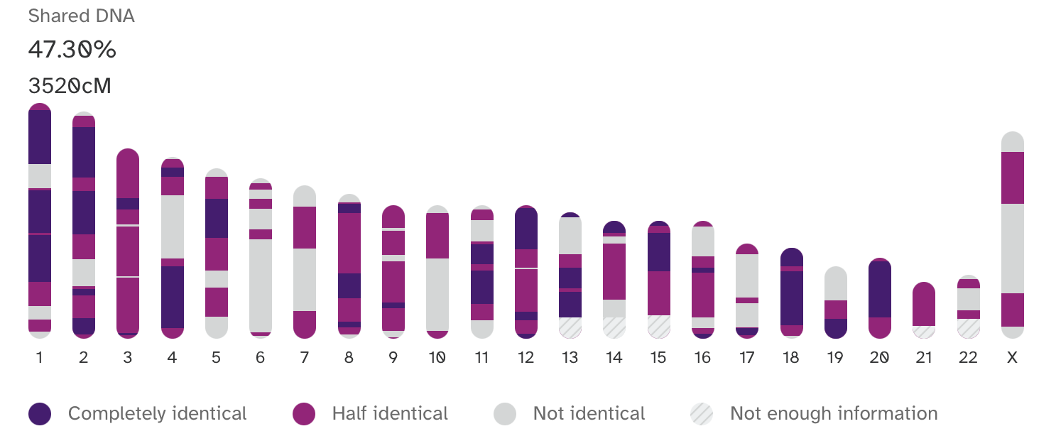
A comparison between my sister’s genome and my own generated by 23andMe.
Between my sister and me, there are regions that we have in common (completely or half identically) and other regions we don’t share. Sequences that are marked as “Completely Identical” represent regions that we both inherited from my mother and my father; we would say that we share two common genetic ancestors (one for each chromosome) in the previous generation. Here, it is important to separate general ancestry from genetic ancestry; whereas ancestry is often used to refer to anyone above you in your family tree, your genetic ancestors are the subset of those individuals from whom you’ve inherited regions of your genome. Continuing further, sequences that are marked as “Half Identical” represent regions where we share a single common genetic ancestor in the previous generation; from this diagram, we cannot discern whether that ancestor is from our mother or father. Lastly, sequences that are marked as “Not Identical” represent regions that require us to look much deeper into the past to identify a common genetic ancestor. Each locus, or position, in our genome reflects a pattern of inheritance that extends back, from generation to generation, to the beginning of life.
By unraveling patterns of sharing between genomes in a population back over multiple generations, researchers can learn about important factors that affect genetic inheritance, such as migration, population size, and natural selection. A lot has been discovered with regards to patterns of inheritance in the over one hundred years since Mendel. Here, I highlight the principles behind coalescent theory and explain the consequences of the random process of genetic inheritance that we observe in our genomes as it plays out over multiple generations.
In 1982, Kingman published “The Coalescent”, describing coalescent theory, a model of inheritance where ancestral lineages in a population are tracked backwards through time, a process independently described by a number of researchers at that time; see Kingman (2000) for a short overview of this history. Let’s start by thinking of a diploid population forward in time. The term “diploid” refers to organisms that have two copies of each locus in their genome; humans, for example, have 23 pairs of chromosomes. To keep things simple, assume that we randomly select two individuals from the populations to parent each offspring in the next generation. At a particular locus, each individual then randomly passes one of their two copies (alleles) on to their offspring. We repeat this random process until the second generation has the same number of individuals as the starting population, thus maintaining a constant population size over time. Below is an example simulation which shows this played out in a population over five generations that we can use to highlight important features of this model.
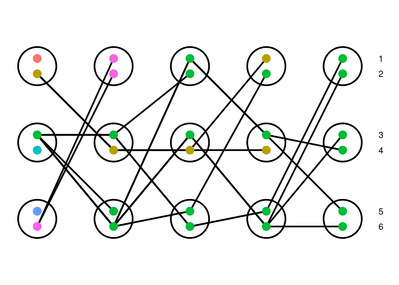
This model is called the neutral Wright-Fisher model. Each allele in the starting population is given a different color to help distinguish them throughout the simulation. All alleles are neutral, meaning that they do not affect the likelihood of producing offspring. Note that this model allows for self-fertilization (selfing), a mechanism where a single individual parents both copies of their offspring’s genome. This mechanism is both grounded in biology (more commonly observed in plants than animals) and helps to simplify calculations within the model.
This is a population of three diploid individuals tracked over five generations (left to right : past to present). Each individual is represented as a circle with two dots, one for each copy of an allele at a locus. Lines connecting copies show how alleles are passed down over time, so that we can track lineages through the generations (by following a line). Due to the randomness of parentage, it is common that not all of the individuals in the parental generation produce offspring in the next generation. Because of this, overtime, certain lineages are lost and others may grow in frequency; this process is known as genetic drift. In the above simulation, the green allele grows in frequency until it is found in every individual in the population. Without mutation, the overall diversity (number of different alleles) of a population with fixed finite size will decrease over time.
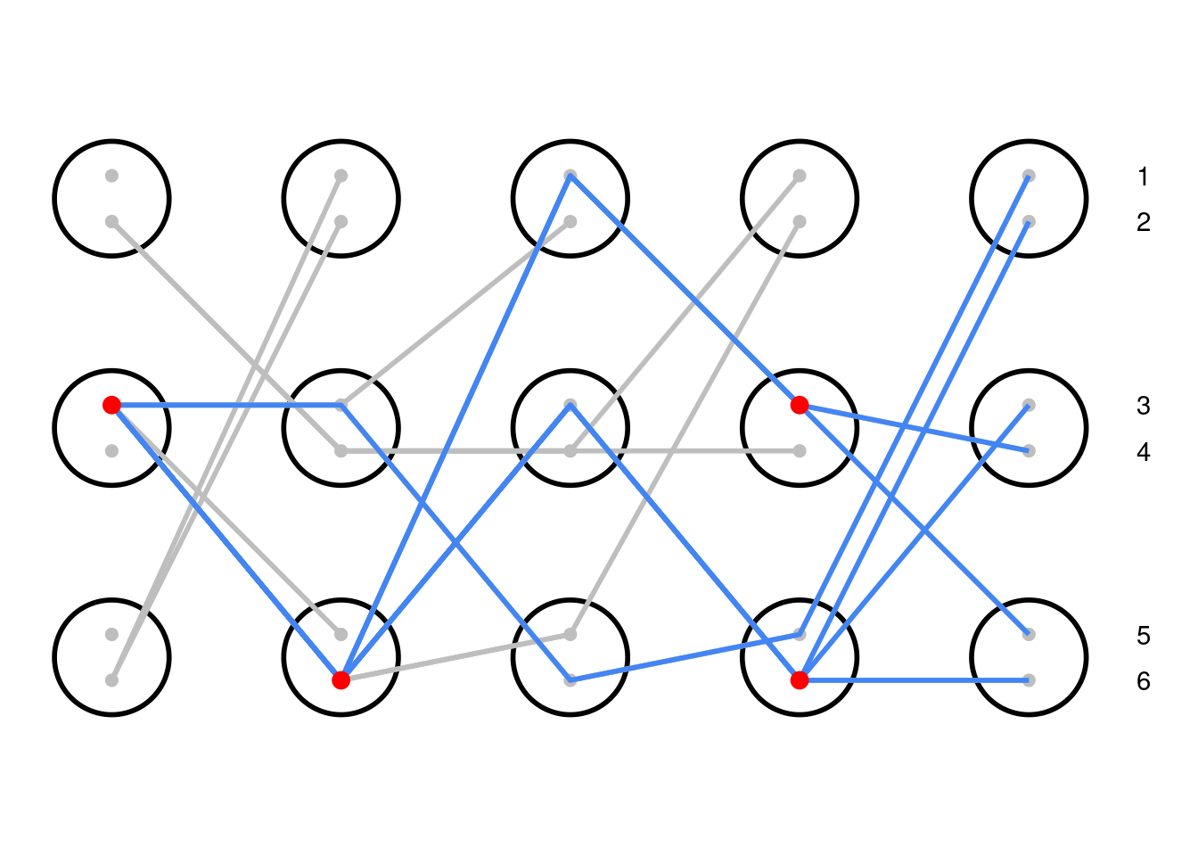
The same simulation as above, now tracing the lineages of the alleles in the present day. All coalescence events are marked with red points. By untangling these lines, we have a genealogical tree that relates all of the alleles.
To understand the coalescent process, we can track present day lineages backwards in time. For example, in the diagram above, you can choose an allele in the present day (on the right) and follow its lineage back through time (from right to left), tracing its blue line all the way back to its ancestors. By tracking multiple lineages at once, we can begin to make sense of the relationships between alleles sampled in the current day. A coalescence event, the namesake of this model, occurs when two copies share a common ancestor. Lineages 4 and 5 from the present generation coalesce one generation in the past; their lines merge into one as we scan to the left. In this simulation, all of the present day lineages share a common ancestor at some point within the past five generations, so we can describe their relationship using a single genealogical tree (shortened to ‘gene tree’ from here on). The root of the tree on the left is the most recent common ancestor of all the lineages, and closely related lineages split more recently on the right side of the tree.
The properties of this gene tree are related to the size of the population; we expect that larger populations will have a gene tree that extends deeper into the past. This is because lineages are less likely to coalesce in a given generation when there are more potential parents due to the larger population size. As this is a random process, it is possible for all lineages to coalesce very quickly, though this is increasingly unlikely at larger population sizes.
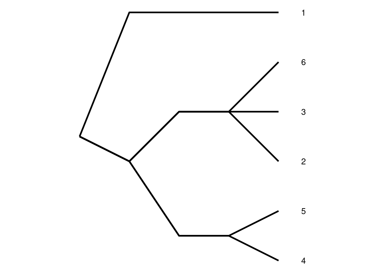
Historically when looking at a family tree, we would not have known which copies each parent passed on to their offspring. A pedigree is a graphical representation of parentage, with no genetic information. Pedigrees are very useful in genetics as they allow us to approximate genetic relatedness without having to directly observe which lineages were passed down from parent to offspring, but importantly, they are not a one-to-one replacement for the original simulation. For a given pedigree, there are many possible simulations, and therefore gene trees, that satisfy the defined relationships between individuals. Below is a simple pedigree of two full siblings, who share both parents, with the corresponding four possible inheritance patterns.
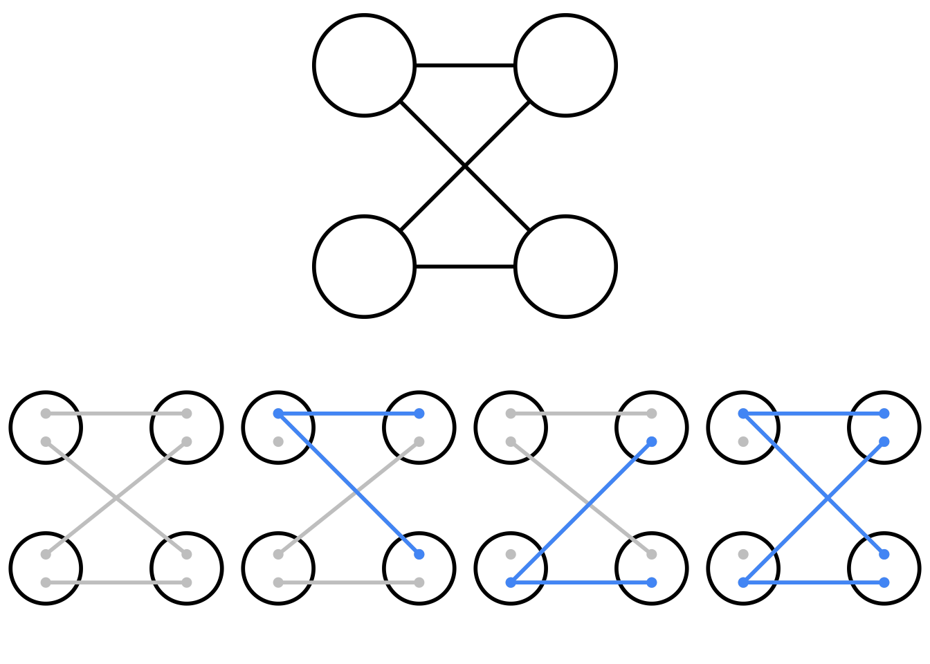
Top: A pedigree of two parents (left) and two offspring (right). Using this diagram alone, it is unknown which allele is passed from parent to offspring. Bottom: The four possible genetic inheritance patterns that correspond to the above pedigree.
Whether you and your (biological) sibling share 0, 1, or 2 alleles at a given locus of your genome is purely chance, reflecting the randomness of Mendelian segregation. Full siblings are expected to share 50% of their autosomal DNA. At any given locus the transmission is random; there is a 25% chance that they share both copies (right diagram), 50% chance that they share one copy (middle two diagrams), and 25% chance that they do not share any copies (left diagram). While in the context of the simulation the randomness of which allele is transmitted by one parent seems trivial it has cascading effects when played out across generations. If we hold the pedigree constant by rerun the randomness of transmission, we generate drastically different gene trees, all of which share the same underlying pedigree. Here is an interactive tool that lets you rerun simulations over a given pedigree to see the changes in possible gene trees1:
But why should we care about this many-to-one relationship between gene trees and pedigrees? Though he didn’t know the mechanisms, Mendel discovered that the alleles underlying many traits assort independently of one another. Today we understand that alleles on different chromosomes will share a pedigree but are independently transmitted to the next generation from each other. Thus loci on different chromosomes are very unlikely to share a gene tree due to this independent assortment (vanishingly unlikely in large populations). Completely independent assortment is equivalent to clicking the “Another Tree From Pedigree” button in the above simulation. Even loci on the same chromosome can be separated through the process of recombination which increases the independence between loci and so reduces the correlation between their gene trees. Because the loci on a chromosome can sort independently from generation to generation, a population’s genetic history cannot be illustrated with a single gene tree. To truly sketch the history, you would need thousands of inter-related gene trees, tracing a whole collection of regions across the genome.
The regions of my genome that I share in common with my sister represent regions with a coalescence event in our parent’s generation. Regions that we don’t share directly in common from the last generation have a much deeper most recent common ancestor; when looking just at these latter regions, my sister is most likely not my closest genetic relative.
In the previous simulations, offspring inherit an identical version of the sequence of their parent’s DNA during reproduction. There’s no genetic variation in these simulations, and so if we were to sequence the individuals in the current day, there’d be no way of reconstructing the gene tree. However, we know that there can be errors in DNA replication (mutations) leading to the development of new alleles, or variants, at a given locus. We can include these mutations in our simulations with two assumptions:
- Mutations are neutral, meaning that they do not affect the relative reproductive success of individuals in the population
- There’s no repeat or back mutation, i.e. mutations that affect precisely the same base pair (this is technically called the infinite sites model)
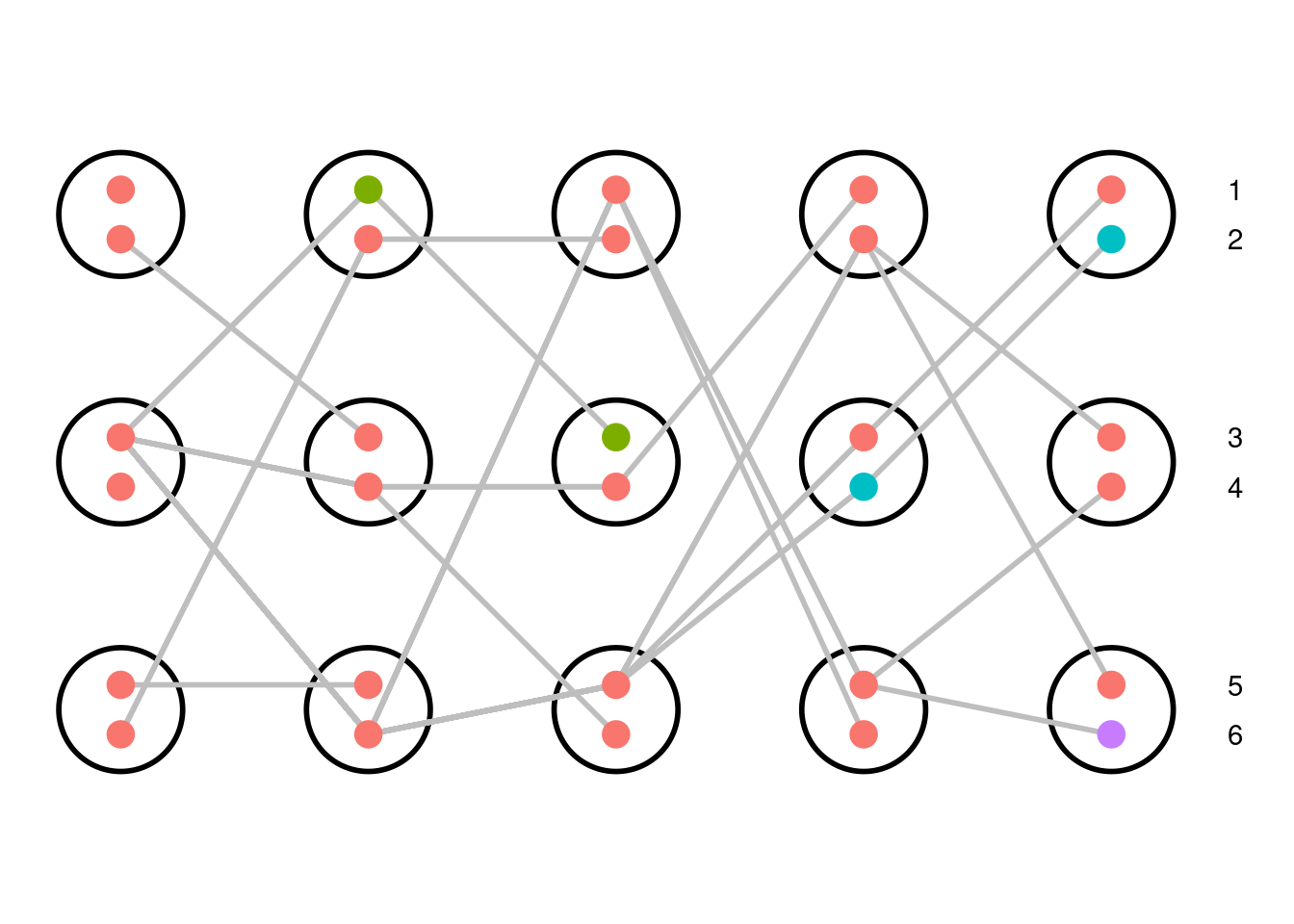
A different simulation of a diploid Wright-Fisher population of three individuals with each variant given a unique color. All alleles in the starting population are the same. Over time, mutations generate new alleles. The mutation rate is set to 0.1 mutations/transmission. The mutation events are added along the gene tree to generate a pseudo-sequence for the gene; only sites that are polymorphic in the present day population are shown.
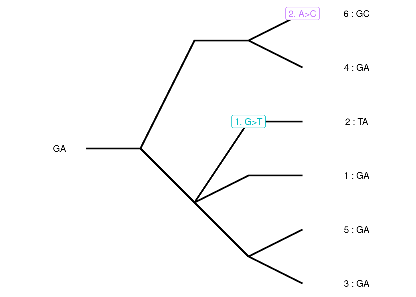
Each allele is given a unique color; there are four gene variants represented in our simulation. Red is the ancestral allele, whereas green, teal, and purple are derived through mutation events in the second, fourth, and fifth generations, respectively. The green allele is lost from the population within two generations whereas the teal and purple alleles persist to the present. These mutation events can be laid on top of the genealogical tree allowing us to more clearly see which individuals are affected by each mutation. Because the blue allele is not represented in the present day population, it is not included on the tree. To generate a pseudo-sequence of this simulated gene, we assign the ancestral and derived variants for each mutation event to nucleotide bases (A, T, G, or C). Every individual then has a sequence of bases corresponding to the mutation events along its ancestral branches. We expect that lineages that are genealogically closely related will also have more similar sequences.
Given the same pedigree, different loci can have very different patterns of transmission, and so very different coalescent trees and very different mutational patterns in their sequences. This is one of the central insights of population genetics. There’s no one tree; a genome is a whole forest.
To wrap up this post, I’ve created an interactive tool that gives you control over many parameters which affect the simulation. Test it out for yourself! All of the code for this post can be found altogether as an R Markdown file here.
All of this work was done in collaboration with my advisor, Dr. Graham Coop, during my first year in the Population Biology Graduate Group at the University of California, Davis. This writing follows up on a series of posts relating to genetic genealogy that can be found on his website, gcbias.org. For a deeper dive into this topic and more, Graham has written an open textbook, Population And Quantitative Genetics, that is freely available for download through the Coop Lab GitHub page.
1Multiple trees from a fixed pedigree figure was partially inspired by a nice figure in Baum and Smith’s Tree Thinking: An Introduction to Phylogenetic Biology. (Tree Thinking: An Introduction to Phylogenetic Biology.— David A. Baum and Stacey D. Smith. 2012. Roberts and Co., Greenwood Village, CO. xx+476 pp. ISBN 9978-1-936221-16-5 $US75 (hardback).)